devNotes 11-5-2016 Guy Fawkes Day

The Inverse Cube Force Law

Here you see three planets. The blue planet is orbiting the Sun in a realistic way: it’s going around an ellipse.

The other two are moving in and out just like the blue planet, so they all stay on the same circle. But they’re moving around this circle at different rates! The green planet is moving faster than the blue one: it completes 3 orbits each time the blue planet goes around once. The red planet isn’t going around at all: it only moves in and out.

What’s going on here?

In 1687, Isaac Newton published his Principia Mathematica. This book is famous, but in Propositions 43–45 of Book I he did something that people didn’t talk about much—until recently. He figured out what extra force, besides gravity, would make a planet move like one of these weird other planets. It turns out an extra force obeying an inverse cube law will do the job!

Let me make this more precise. We’re only interested in ‘central forces’ here. A central force is one that only pushes a particle towards or away from some chosen point, and only depends on the particle’s distance from that point. In Newton’s theory, gravity is a central force obeying an inverse square law:

$F(r) = - \displaystyle{ \frac{a}{r^2} }$

for some constant $a.$ But he considered adding an extra central force obeying an inverse cube law:

$F(r) = - \displaystyle{ \frac{a}{r^2} + \frac{b}{r^3} }$

He showed that if you do this, for any motion of a particle in the force of gravity you can find a motion of a particle in gravity plus this extra force, where the distance $r(t)$ is the same, but the angle $\theta(t)$ is not.

In fact Newton did more. He showed that if we start with any central force, adding an inverse cube force has this effect.

There’s a very long page about this on Wikipedia:

• Newton’s theorem of revolving orbits, Wikipedia.

I haven’t fully understood all of this, but it instantly makes me think of three other things I know about the inverse cube force law, which are probably related. So maybe you can help me figure out the relationship.

The first, and simplest, is this. Suppose we have a particle in a central force. It will move in a plane, so we can use polar coordinates $r, \theta$ to describe its position. We can describe the force away from the origin as a function $F(r).$ Then the radial part of the particle’s motion obeys this equation:

$\displaystyle{ m \ddot r = F(r) + \frac{L^2}{mr^3} }$

where $L$ is the magnitude of particle’s angular momentum.

So, angular momentum acts to provide a ‘fictitious force’ pushing the particle out, which one might call the centrifugal force. And this force obeys an inverse cube force law!

Furthermore, thanks to the formula above, it’s pretty obvious that if you change $L$ but also add a precisely compensating inverse cube force, the value of $\ddot r$ will be unchanged! So, we can set things up so that the particle’s radial motion will be unchanged. But its angular motion will be different, since it has a different angular momentum. This explains Newton’s observation.

It’s often handy to write a central force in terms of a potential:

$F(r) = -V'(r)$

Then we can make up an extra potential responsible for the centrifugal force, and combine it with the actual potential $V$ into a so-called effective potential:

$\displaystyle{ U(r) = V(r) + \frac{L^2}{2mr^2} }$

The particle’s radial motion then obeys a simple equation:

$\ddot{r} = - U'(r)$

For a particle in gravity, where the force obeys an inverse square law and $V$ is proportional to $-1/r,$ the effective potential might look like this:

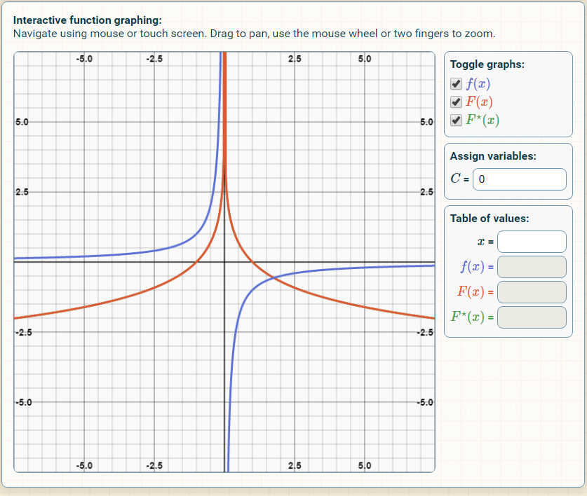
This is the graph of

$\displaystyle{ U(r) = -\frac{4}{r} + \frac{1}{r^2} }$

If you’re used to particles rolling around in potentials, you can easily see that a particle with not too much energy will move back and forth, never making it to $r = 0$ or $r = \infty.$ This corresponds to an elliptical orbit. Give it more energy and the particle can escape to infinity, but it will never hit the origin. The repulsive ‘centrifugal force’ always overwhelms the attraction of gravity near the origin, at least if the angular momentum is nonzero.

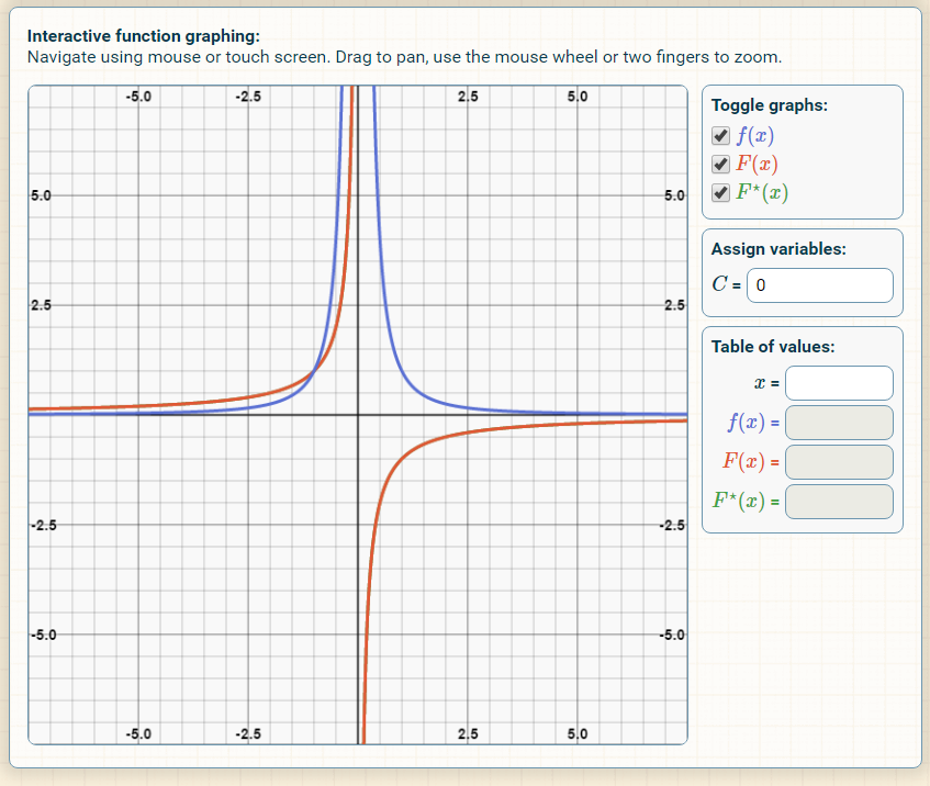
On the other hand, suppose we have a particle moving in an attractive inverse cube force! Then the potential is proportional to $1/r^2,$ so the effective potential is

$\displaystyle{ U(r) = \frac{c}{r^2} + \frac{L^2}{mr^2} }$

where $c$ is negative for an attractive force. If this attractive force is big enough, namely

$\displaystyle{ c < -\frac{L^2}{m} }$

then this force can exceed the centrifugal force, and the particle can fall in to $r = 0.$

If we keep track of the angular coordinate $\theta,$ we can see what’s really going on. The particle is spiraling in to its doom, hitting the origin in a finite amount of time!

This should remind you of a black hole, and indeed something similar happens there, but even more drastic:

• Schwarzschild geodesics: effective radial potential energy, Wikipedia.

For a nonrotating uncharged black hole, the effective potential has three terms. Like Newtonian gravity it has an attractive $-1/r$ term and a repulsive $1/r^2$ term. But it also has an attractive term $-1/r^3$ term! In other words, it’s as if on top of Newtonian gravity, we had another attractive force obeying an inverse fourth power law! This overwhelms the others at short distances, so if you get too close to a black hole, you spiral in to your doom.

For example, a black hole can have an effective potential like this:

But back to inverse cube force laws! I know two more things about them. A while back I discussed how a particle in an inverse square force can be reinterpreted as a harmonic oscillator:

• Planets in the fourth dimension, Azimuth.

There are many ways to think about this, and apparently the idea in some form goes all the way back to Newton! It involves a sneaky way to take a particle in a potential

$\displaystyle{ V(r) \propto r^{-1} }$

and think of it as moving around in the complex plane. Then if you squareits position—thought of as a complex number—and cleverly reparametrize time, you get a particle moving in a potential

$\displaystyle{ V(r) \propto r^2 }$

This amazing trick can be generalized! A particle in a potential

$\displaystyle{ V(r) \propto r^p }$

can transformed to a particle in a potential

$\displaystyle{ V(r) \propto r^q }$

$(p+2)(q+2) = 4$

A good description is here:

• Rachel W. Hall and Krešimir Josić, Planetary motion and the duality of force laws, SIAM Review 42 (2000), 115–124.

This trick transforms particles in $r^p$ potentials with $p$ ranging between $-2$ and $+\infty$ to $r^q$ potentials with $q$ ranging between $+\infty$ and $-2.$ It’s like a see-saw: when $p$ is small, $q$ is big, and vice versa.

But you’ll notice this trick doesn’t actually work at $p = -2,$ the case that corresponds to the inverse cube force law. The problem is that $p + 2 = 0$ in this case, so we can’t find $q$ with $(p+2)(q+2) = 4.$

So, the inverse cube force is special in three ways: it’s the one that you can add on to any force to get solutions with the same radial motion but different angular motion, it’s the one that naturally describes the ‘centrifugal force’, and it’s the one that doesn’t have a partner! We’ve seen how the first two ways are secretly the same. I don’t know about the third, but I’m hopeful.

Quantum aspects

Finally, here’s a fourth way in which the inverse cube law is special. This shows up most visibly in quantum mechanics… and this is what got me interested in this business in the first place.

You see, I’m writing a paper called ‘Struggles with the continuum’, which discusses problems in analysis that arise when you try to make some of our favorite theories of physics make sense. The inverse square force law poses interesting problems of this sort, which I plan to discuss. But I started wanting to compare the inverse cube force law, just so people can see things that go wrong in this case, and not take our successes with the inverse square law for granted.

Unfortunately a huge digression on the inverse cube force law would be out of place in that paper. So, I’m offloading some of that material to here.

In quantum mechanics, a particle moving in an inverse cube force law has a Hamiltonian like this:

$H = -\nabla^2 + c r^{-2}$

The first term describes the kinetic energy, while the second describes the potential energy. I’m setting $\hbar = 1$ and $2m = 1$ to remove some clutter that doesn’t really affect the key issues.

To see how strange this Hamiltonian is, let me compare an easier case. If $p < 2,$ the Hamiltonian

$H = -\nabla^2 + c r^{-p}$

is essentially self-adjoint on $C_0^\infty(\mathbb{R}^3 - \{0\}),$ which is the space of compactly supported smooth functions on 3d Euclidean space minus the origin. What this means is that first of all, $H$ is defined on this domain: it maps functions in this domain to functions in $L^2(\mathbb{R}^3)$ . But more importantly, it means we can uniquely extend $H$ from this domain to a self-adjoint operator on some larger domain. In quantum physics, we want our Hamiltonians to be self-adjoint. So, this fact is good.

Proving this fact is fairly hard! It uses something called the Kato–Lax–Milgram–Nelson theorem together with this beautiful inequality:

$\displaystyle{ \int_{\mathbb{R}^3} \frac{1}{4r^2} |\psi(x)|^2 \,d^3 x \le \int_{\mathbb{R}^3} |\nabla \psi(x)|^2 \,d^3 x }$

for any $\psi\in C_0^\infty(\mathbb{R}^3).$

If you think hard, you can see this inequality is actually a fact about the quantum mechanics of the inverse cube law! It says that if $c \ge -1/4,$ the energy of a quantum particle in the potential $c r^{-2}$ is bounded below. And in a sense, this inequality is optimal: if $c < -1/4$ , the energy is not bounded below. This is the quantum version of how a classical particle can spiral in to its doom in an attractive inverse cube law, if it doesn’t have enough angular momentum. But it’s subtly and mysteriously different.

You may wonder how this inequality is used to prove good things about potentials that are ‘less singular’ than the $c r^{-2}$ potential: that is, potentials $c r^{-p}$ with $p < 2.$ For that, you have to use some tricks that I don’t want to explain here. I also don’t want to prove this inequality, or explain why its optimal! You can find most of this in some old course notes of mine:

• John Baez, Quantum Theory and Analysis, 1989.

See especially section 15.

But it’s pretty easy to see how this inequality implies things about the expected energy of a quantum particle in the potential $c r^{-2}$ . So let’s do that.

In this potential, the expected energy of a state $\psi$ is:

$\displaystyle{ \langle \psi, H \psi \rangle = \int_{\mathbb{R}^3} \overline\psi(x)\, (-\nabla^2 + c r^{-2})\psi(x) \, d^3 x }$

Doing an integration by parts, this gives:

$\displaystyle{ \langle \psi, H \psi \rangle = \int_{\mathbb{R}^3} |\nabla \psi(x)|^2 + cr^{-2} |\psi(x)|^2 \,d^3 x }$

The inequality I showed you says precisely that when $c = -1/4,$ this is greater than or equal to zero. So, the expected energy is actually nonnegative in this case! And making $c$ greater than $-1/4$ only makes the expected energy bigger.

Note that in classical mechanics, the energy of a particle in this potential ceases to be bounded below as soon as $c < 0.$ Quantum mechanics is different because of the uncertainty principle! To get a lot of negative potential energy, the particle’s wavefunction must be squished near the origin, but that gives it kinetic energy.

It turns out that the Hamiltonian for a quantum particle in an inverse cube force law has exquisitely subtle and tricky behavior. Many people have written about it, running into ‘paradoxes’ when they weren’t careful enough. Only rather recently have things been straightened out.

For starters, the Hamiltonian for this kind of particle

$H = -\nabla^2 + c r^{-2}$

has different behaviors depending on $c.$ Obviously the force is attractive when $c > 0$ and repulsive when $c < 0,$ but that’s not the only thing that matters! Here’s a summary:

• $c \ge 3/4.$ In this case $H$ is essentially self-adjoint on $C_0^\infty(\mathbb{R}^3 - \{0\}).$ So, it admits a unique self-adjoint extension and there’s no ambiguity about this case.

• $c < 3/4.$ In this case $H$ is not essentially self-adjoint on $C_0^\infty(\mathbb{R}^3 - \{0\}).$ In fact, it admits more than one self-adjoint extension! This means that we need extra input from physics to choose the Hamiltonian in this case. It turns out that we need to say what happens when the particle hits the singularity at $r = 0.$ This is a long and fascinating story that I just learned yesterday.

• $c \ge -1/4.$ In this case the expected energy $\langle \psi, H \psi \rangle$ is bounded below for $\psi \in C_0^\infty(\mathbb{R}^3 - \{0\}).$ It turns out that whenever we have a Hamiltonian that is bounded below, even if there is not a unique self-adjoint extension, there exists a canonical ‘best choice’ of self-adjoint extension, called the Friedrichs extension. I explain this in my course notes.

• $c < -1/4.$ In this case the expected energy is not bounded below, so we don’t have the Friedrichs extension to help us choose which self-adjoint extension is ‘best’.

To go all the way down this rabbit hole, I recommend these two papers:

• Sarang Gopalakrishnan, Self-Adjointness and the Renormalization of Singular Potentials, B.A. Thesis, Amherst College.

• D. M. Gitman, I. V. Tyutin and B. L. Voronov, Self-adjoint extensions and spectral analysis in the Calogero problem, Jour. Phys. A 43 (2010), 145205.

The first is good for a broad overview of problems associated to singular potentials such as the inverse cube force law; there is attention to mathematical rigor the focus is on physical insight. The second is good if you want—as I wanted—to really get to the bottom of the inverse cube force law in quantum mechanics. Both have lots of references.

Also, both point out a crucial fact I haven’t mentioned yet: in quantum mechanics the inverse cube force law is special because, naively, at leastit has a kind of symmetry under rescaling! You can see this from the formula

$H = -\nabla^2 + cr^{-2}$

by noting that both the Laplacian and $r^{-2}$ have units of length^-2. So, they both transform in the same way under rescaling: if you take any smooth function $\psi$ , apply $H$ and then expand the result by a factor of $k,$ you get $k^2$ times what you get if you do those operations in the other order.

In particular, this means that if you have a smooth eigenfunction of $H$ with eigenvalue $\lambda,$ you will also have one with eigenfunction $k^2 \lambda$ for any $k > 0.$ And if your original eigenfunction was normalizable, so will be the new one!

With some calculation you can show that when $c \le -1/4,$ the Hamiltonian $H$ has a smooth normalizable eigenfunction with a negative eigenvalue. In fact it’s spherically symmetric, so finding it is not so terribly hard. But this instantly implies that $H$ has smooth normalizable eigenfunctions with any negative eigenvalue.

This implies various things, some terrifying. First of all, it means that $H$ is not bounded below, at least not on the space of smooth normalizable functions. A similar but more delicate scaling argument shows that it’s also not bounded below on $C_0^\infty(\mathbb{R}^3 - \{0\}),$ as I claimed earlier.

This is scary but not terrifying: it simply means that when $c \le -1/4,$ the potential is too strongly negative for the Hamiltonian to be bounded below.

The terrifying part is this: we’re getting uncountably many normalizable eigenfunctions, all with different eigenvalues, one for each choice of $k.$ A self-adjoint operator on a countable-dimensional Hilbert space like $L^2(\mathbb{R}^3)$ can’t have uncountably many normalizable eigenvectors with different eigenvalues, since then they’d all be orthogonal to each other, and that’s too many orthogonal vectors to fit in a Hilbert space of countable dimension!

This sounds like a paradox, but it’s not. These functions are not all orthogonal, and they’re not all eigenfunctions of a self-adjoint operator. You see, the operator $H$ is not self-adjoint on the domain we’ve chosen, the space of all smooth functions in $L^2(\mathbb{R}^3).$ We can carefully choose a domain to get a self-adjoint operator… but it turns out there are many ways to do it.

Intriguingly, in most cases this choice breaks the naive dilation symmetry. So, we’re getting what physicists call an ‘anomaly’: a symmetry of a classical system that fails to give a symmetry of the corresponding quantum system.

Of course, if you’ve made it this far, you probably want to understand what the different choices of Hamiltonian for a particle in an inverse cube force law actually mean, physically. The idea seems to be that they say how the particle changes phase when it hits the singularity at $r = 0$ and bounces back out.

(Why does it bounce back out? Well, if it didn’t, time evolution would not be unitary, so it would not be described by a self-adjoint Hamiltonian! We could try to describe the physics of a quantum particle that does notcome back out when it hits the singularity, and I believe people have tried, but this requires a different set of mathematical tools.)

For a detailed analysis of this, it seems one should take Schrödinger’s equation and do a separation of variables into the angular part and the radial part:

$\psi(r,\theta,\phi) = \Psi(r) \Phi(\theta,\phi)$

For each choice of $\ell = 0,1,2,\dots$ one gets a space of spherical harmonics that one can use for the angular part $\Phi.$ The interesting part is the radial part, $\Psi.$ Here it is helpful to make a change of variables

$u(r) = \Psi(r)/r$

At least naively, Schrödinger’s equation for the particle in the $cr^{-2}$ potential then becomes

$\displaystyle{ \frac{d}{dt} u = -iH u }$

where

$\displaystyle{ H = -\frac{d^2}{dr^2} + \frac{c + \ell(\ell+1)}{r^2} }$

Beware: I keep calling all sorts of different but related Hamiltonians $H,$ and this one is for the radial part of the dynamics of a quantum particle in an inverse cube force. As we’ve seen before in the classical case, the centrifugal force and the inverse cube force join forces in an ‘effective potential’

$\displaystyle{ U(r) = kr^{-2} }$

where

$k = c + \ell(\ell+1)$

So, we have reduced the problem to that of a particle on the open half-line $(0,\infty)$ moving in the potential $kr^{-2}.$ The Hamiltonian for this problem:

$\displaystyle{ H = -\frac{d^2}{dr^2} + \frac{k}{r^2} }$

is called the Calogero Hamiltonian. Needless to say, it has fascinating and somewhat scary properties, since to make it into a bona fide self-adjoint operator, we must make some choice about what happens when the particle hits $r = 0.$ The formula above does not really specify the Hamiltonian.

This is more or less where Gitman, Tyutin and Voronov begin their analysis, after a long and pleasant review of the problem. They describe all the possible choices of self-adjoint operator that are allowed. The answer depends on the values of $k,$ but very crudely, the choice says something like how the phase of your particle changes when it bounces off the singularity. Most choices break the dilation invariance of the problem. But intriguingly, some choices retain invariance under a discrete subgroup of dilations!

So, the rabbit hole of the inverse cube force law goes quite deep, and I expect I haven’t quite gotten to the bottom yet. The problem may seem pathological, verging on pointless. But the math is fascinating, and it’s a great testing-ground for ideas in quantum mechanics—very manageable compared to deeper subjects like quantum field theory, which are riddled with their own pathologies. Finally, the connection between the inverse cube force law and centrifugal force makes me think it’s not a mere curiosity.

In four dimensions

It’s a bit odd to study the inverse cube force law in 3-dimensonal space, since Newtonian gravity and the electrostatic force would actually obey an inverse cube law in 4-dimensional space. For the classical 2-body problem it doesn’t matter much whether you’re in 3d or 4d space, since the motion stays on the plane. But for quantum 2-body problem it makes more of a difference!

Just for the record, let me say how the quantum 2-body problem works in 4 dimensions. As before, we can work in the center of mass frame and consider this Hamiltonian:

$H = -\nabla^2 + c r^{-2}$

And as before, the behavior of this Hamiltonian depends on $c.$ Here’s the story this time:

• $c \ge 0.$ In this case $H$ is essentially self-adjoint on $C_0^\infty(\mathbb{R}^4 - \{0\}).$ So, it admits a unique self-adjoint extension and there’s no ambiguity about this case.

• $c < 0.$ In this case $H$ is not essentially self-adjoint on $C_0^\infty(\mathbb{R}^4 - \{0\}).$

• $c \ge -1.$ In this case the expected energy $\langle \psi, H \psi \rangle$ is bounded below for $\psi \in C_0^\infty(\mathbb{R}^3 - \{0\}).$ So, there is exists a canonical ‘best choice’ of self-adjoint extension, called the Friedrichs extension.

• $c < -1.$ In this case the expected energy is not bounded below, so we don’t have the Friedrichs extension to help us choose which self-adjoint extension is ‘best’.

I’ve been assured these are correct by Barry Simon, and a lot of this material will appear in Section 7.4 of his book:

• Barry Simon, A Comprehensive Course in Analysis, Part 4: Operator Theory, American Mathematical Society, Providence, RI, 2015.

Notes

The animation was made by ‘WillowW’ and placed on Wikicommons. It’s one of a number that appears in this Wikipedia article:

• Newton’s theorem of revolving orbits, Wikipedia.

I made the graphs using the free online Desmos graphing calculator.

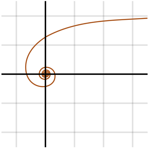
The picture of a spiral was made by ‘Anarkman’ and ‘Pbroks13’ and placed on Wikicommons; it appears in

• Hyperbolic spiral, Wikipedia.

The hyperbolic spiral is one of three kinds of orbits that are possible in an inverse cube force law. They are vaguely analogous to ellipses, hyperbolas and parabolas, but there are actually no bound orbits except perfect circles. The three kinds are called Cotes’s spirals. In polar coordinates, they are:

• the epispiral:

$\displaystyle{ \frac{1}{r} = A \cos\left( k\theta + \varepsilon \right) }$

• the hyperbolic spiral:

$\displaystyle{ \frac{1}{r} = A \cosh\left( k\theta + \varepsilon \right) }$

• the Poinsot spiral:

$\displaystyle{ \frac{1}{r} = A \theta + \varepsilon }$

gfjmfgfmjgjm9

ghfmhgmhmh

Integral

ghfmhgmhmh

Comparing Velocity to Particle Radius to Attractor

#pragma kernel CSMain

// Thread group size 
#define thread_group_size_x 32
#define thread_group_size_y 1
#define thread_group_size_z 1

struct Particle 
{
    float3      position;  
    float3      velocity; 
    float3      position_last;
};

int app_mode;

float  time;
float  pi;

float deltaTime;
float damping;									
float3 base;										// HANDLE.
float3 orbit;										// BOB
float targetStrength;								// POWER MAG
float orbit_weighting;                              // POWER RATIO BETWEEN HANDLE AND BOB
float radius_of_action;                             // RADIUS OF TROUGH / MOTE :) around ATTRACTOR
float zero_mirror_radius;

int attractor_Count;
float3 att_0;										
float3 att_1;
float3 att_2;										
float3 att_3;

float3 att_4;										
float3 att_5;
float3 att_6;										
float3 att_7;

float3 att_8;										
float3 att_9;
float3 att_10;										
float3 att_11;

float3 att_12;										
float3 att_13;
float3 att_14;										
float3 att_15;

float3 att_16;										
float3 att_17;
float3 att_18;										
float3 att_19;
	
float constVel;                                     

RWStructuredBuffer <Particle> particles;

[numthreads(thread_group_size_x, thread_group_size_y, thread_group_size_z )]

void CSMain ( uint3 Gid : SV_GroupID, uint3 DTid : SV_DispatchThreadID, uint3 GTid : SV_GroupThreadID, uint GI : SV_GroupIndex )        
{
    int index = DTid.x;
    //int index = DTid.x + DTid.y * thread_group_size_x * 32;
   
    if(app_mode == 0) //Platonics Mode
    {
        float3 velTemp = particles[index].velocity;

        float3 vZero;
        vZero.x = 0;
        vZero.y = 0;
        vZero.z = 0;

        float3 pN_pL_dir = normalize((particles[index].position - particles[index].position_last));
        float  pN_pL_dist = distance(particles[index].position, particles[index].position_last);  
            
        float3 deltVel;
        float dV_Len;
        float dV_Last_Len;   
             
        if(attractor_Count == 1 || attractor_Count == 2 || attractor_Count == 3 )
        {
            float3 att_0_Dir  = normalize((att_0 - particles[index].position));
            float  att_0_dist = distance(att_0, particles[index].position);
            deltVel = targetStrength * att_0_Dir * deltaTime / att_0_dist;
            if(att_0_dist > zero_mirror_radius*length(particles[index].velocity))
            {

                velTemp += deltVel;
                //particles[index].position_last = deltVel;
            }
            else
            {
                //velTemp += particles[index].position_last;
            }

            if(attractor_Count == 2 || attractor_Count == 3 )
            {
                float3 att_1_Dir = normalize((att_1 - particles[index].position));
                float att_1_dist = distance(att_1, particles[index].position);
                
               if(att_1_dist > zero_mirror_radius*length(particles[index].velocity))
               {
                    deltVel = targetStrength * att_1_Dir * deltaTime / att_1_dist;
                    velTemp += deltVel;
                    //particles[index].position_last = deltVel;
                }
                else
                {
                    //velTemp += particles[index].position_last;
                }

The Question is:

Does the Universe exist in Time?

Does time exist in the Universe?

002a